GIS II: Lab 6- Data Normalization, Geocoding, and Error Assessment

Goal

The goal of this lab was to learn how to geocode by geocoding the locations of sand mines in Wisconsin and comparing the results to the actual locations of the mines.  

The data used for this lab came from the Wisconsin DNR, but the data was incredibly messy.  There were different types of street addresses and PLSS addresses.  Some locations had both types while some only had one or the other.  We were all assigned 16 mines out of 129 and were to normalize the data.  When the normalization was done, the table was then imported into the geocoding toolbar in ArcMap.  After the 16 mines were geocoded, the actual mine locations were imported and compared to the ones we had geocoded.  We also had to compare our personal 16 mines with those of our classmates who had the same mines.  The final step was to create an error table in order to see how well we had geocoded our mines compared to where the actual mine locations were.

Methods

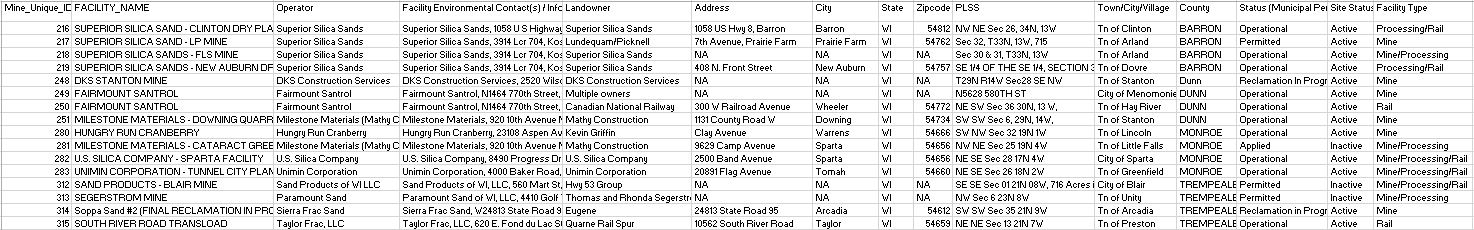
The first step to this lab was to figure out which 16 mines were ours.  We then had to create a new table with normalized data in order for it to be imported into ArcMap.  My 16 mines had their data entered quite differently so normalization was definitely needed.  Below in Figure 1.1 is how I received the data.  Figure 1.2 is the data after I had normalized it.

Figure 1.1: How I received the data from the DNR.

Figure 1.2: Normalized data for my 16 mines.

After normalizing my data it was time to geocode the addresses in ArcMap.  I entered the table that I wanted geocoded and 11 of my addresses were matched, but the other 5 were unmatched.  I added the points to the map along with an imagery base map in order to make it easier to see if the mines were in the correct locations.  I went through the 11 matched addresses first in order to make sure they were matched to the correct addresses.  In order to do this, I zoomed into each matched location to see if I could see the sand mine in that general area.  For the most of them the address was right and I could see the sand mine on the base map.  There were a few, though, that were in completely wrong areas.  In order to fix these I had to look at their PLSS addresses.  I added the Wisconsin townships and sections layers in order to better locate where these sand mines were.  For the 5 that were unmatched I also had to look at the PLSS address.  These sand mines either did not have a street address or their PLSS address was not normalized enough for ArcMap to figure it out.  It took quite a bit of time of struggling to estimate where these mines were, but I eventually geocoded all 16 mines.

Next I need to compare my personal geocoded mines with their actual locations and with my classmates geocoded mines.  The actual locations of the mines layer imported with all 129 mines, though, so I needed to select just my 16 in order to get a better understanding of where my mines actually were.  I created a new layer for the actual locations and did the same with my classmates who geocoded the same mines as I did.  I compared my mines with the actual locations in Figure 2.1 below.  In Figure 2.2 I compared my geocoded mines with my classmates mines.

Figure 2.1: My geocoded mines compared to their actual locations.

Figure 2.1: My geocoded mines compared to my classmates geocoded mines.

For the most part, most of my mines were in the right location compared to their actual locations and to my classmates mines.  I created an error table comparing how off I was in meters compared to the actual locations and classmates locations.  Only about three were completely off, which was my error.  For the rest, they are all in the same location.  The numbers may seem to look like I was completely off, but the scenario was usually that I was in the right location, but I just put my point down the street or a few meters away from where the DNR and my classmates had put theirs.  If the numbers are below 2,500 meters it means that I had the right location, but the points are in different spots.  The table is pictured below in Figure 3.

Figure 3: Meters my mines were off from actual locations and classmates mines.

Discussion

When I first received the data, I could tell there were many errors with all of the mines in the table.  There are three types of errors that can happen with data: gross errors, systematic errors, and random errors.  The first type of error that I saw right away with this data was gross error.  These are just mistakes or oversights that may have happened.  These can be fixed by properly training employees and those collecting the data that the information should be collected in a standardized procedure.  It's obvious that the data was not collected in this manner.  Systematic errors weren't as prominent as gross errors.  This type of error is typically from instruments not being properly calibrated and from changing environmental conditions.  These were a possibility, but were not seen in the data.  Random errors are the leftover ones that don't fit into the first two categories.  All data has random errors, but they are often small errors and can be easily fixed.  I believe these errors were either fixed before the data was received or I just didn't notice them.  

There is also inherent and operational errors.  Inherent errors occur because real world phenomena cannot be accurately represented in data and models.  They are generalized and are sometimes incomplete. The real world is too complicated to represent in data and modeling.  Operational errors occur when the data is actually being collected.  This is also known as user error.  These two types of error occur in all data which means these are present in the data used for this lab.  This leads to the question, how do we know what is accurate data and what is not?  By following set rules and guidelines while collecting and processing data we can ensure that our data will keep it's integrity.  If all data were to be collected and dispersed like the DNR mine data, then many errors would have to be dealt with and much more work would be needed in order to create accurate results.  By following standardized procedures, we can skip unnecessary errors and collect and produce accurate data.

Conclusions

This lab was quite frustrating, but in the end I learned the importance of collecting standardized data.  Collecting data that is organized and understandable is vital in producing accurate findings.  We can't use data that is full of errors and expect to get reliable results.  It is very important to be vigilant throughout the whole scientific process.

Sources

http://resources.arcgis.com/en/help/

Lo, C.P., and Albert K. W. Yeung. "Chapter 4: Data Quality and Data Standards." Concepts and Techniques of Geographic Information Systems. Upper Saddle River, NJ: Pearson Prentice Hall, 2003. 103-134. Print.

GIS II: Lab 2- Data Downloading, Interoperability, and Working with Projections in Python

Goal

The main purpose of the lab was to become familiar with python and downloading data in an organized fashion.  Below in figure 1 is an example of the general flow of this lab including both parts 1 and 2.

Figure 1: General workflow of lab 2.

Part 1: Data Downloading, Interoperability, and Working with Projections

In order to begin this lab, a large amount of data needed to be downloaded.  This data came from US Department of Transportation, USGS National Map Viewer (National Land Cover Data), USDA Geospatial Data Gateway, Trempealeau County land records, and the USDA NRCS web soil survey.  This was such a great amount of data that it needed to be done in a very organized fashion in order not to lose it or the integrity of the data.  In order to do this I created a file folder for each website that I downloaded data from.  From here the data needed to be unzipped and imported into the correct folders.  After this, I checked the data to make sure it was accurate.  I joined the necessary tables, merged data, and once again made sure it was accurate. I collected information about all of the data that was downloaded and it is shown in figure 2 below.

Figure 2: Information about data download in part 1.

Part 2: Working in Python

The goal for the second part of the lab was to become familiar with python script and apply those skills in order to create maps relevant to this project.  There were three rasters we had to clip to the outline of Trempealeau county.  The python script for that was used for this is in the previous blog post (GIS II: Python).  Writing the script took a of effort before it all worked out, but after it all worked I imported the three rasters now in the shape of Trempealeau county into ArcMap.  The final product of this lab is in figure 3 below.

Figure 3: Trempealeau county maps final product.

Conclusions

The data that was downloaded in part 1 of this lab was very different from each other.  Some of the metadata was complete and informative and others were lacking in those fields.  I learned the importance of organizing my data from the start and continued that process throughout the lab.  In part 2, I really dove into the python process.  I eventually found myself understanding the ins and outs of the whole program, though many frustrating hours had to go into that before the understanding came.  I found that writing the script was actually easier and less confusing at times rather than manually running the tools in ArcMap.  I hope to use python more often after now learning the basics of the program.

Sources

NLCD 2011 Land Cover Metadata:

 https://www.sciencebase.gov/catalog/item/550c31ebe4b02e76d759d4cf

NLCD 2011 Land Cover data info:

http://www.mrlc.gov/nlcd2011.php

NLCD product legend:

http://www.mrlc.gov/nlcd06_leg.php

Elevation metadata (northern):

https://www.sciencebase.gov/catalog/item/5311fa5de4b0d490f4ab4626

Elevation metadata (southern):

https://www.sciencebase.gov/catalog/item/5311fa6be4b0d490f4ab47ca

GIS II: Python

Goal and Background

The objective for this post is to show the python scripting that I created in order to make rasters specifically for Lab 2.  The python script I created is shown below in Figure 1.  The rasters I created are of Trempealeau county.  They will show elevation, land cover, and crop cover.

Figure 1: Python script for lab 2.

GIS II: Sand Mining in Western Wisconsin

Goal

The purpose of this post is to give background information on sand mining in Wisconsin.  This is in order to prepare for an upcoming lab being done in Geography 337- GIS II.  

Background

Frac sand mining (also known as hydraulic fracturing)  in Wisconsin has been going on for about 100 years now and has many different uses.  Sand mining is used for creating filter beds for drinking water and waste water treatment, glass manufacturing, uses in the petroleum industry, and more.  Frac sand is quartz sand with a specific grain size and shape and is suspended in fluid.  The frac sand is used for extracting natural gas and crude oil from rock formations.  The sand is injected into fractures of the earth which are closed or not fully opened.  The sand grains open up the fractures in order to extract the oil and gas within them.  

Frac sand mining has only recently boomed in Wisconsin in the past five or so years.  This industry is huge in Wisconsin because of the sand found in mostly the western half of the state.  The recent boom in the industry has caused any problems for Wisconsin and other states in the Midwest being used for their sand.  Wisconsin has very few laws set in place when it comes to sand mining and these laws are very infrequently enforced.  Sand mining also has great environmental hazards that come along with it.  It causes air pollution, water pollution, erosion, and more.  This industry has pros and cons, but does not have enough laws in order to keep those in check.

Figure 1: Sand mining in Wisconsin.

Pictured above in Figure 1 is a map of sand mining area in Wisconsin and also areas where the sand is found throughout Wisconsin.  Since this map was created in 2012, many news frac sand mining sites have been created throughout the state.

GIS Applications

There are many applications when GIS is used in frac sand mining.  For example, we could create a map similar to the one pictured above of where sand mining sites are throughout the state.  We could then add data about where air and water pollution are the greatest throughout the state and see if the data displays a correlation to the two.  GIS data can also help us decide as to where the next ideal sand mining site could be place in the state.  We can look at data on where mining sites already exist and where environmental hazards are greatest to decide where to go next.  There are many applications where GIS is used in frac sand mining, whether they are seen as good or bad.

Sources

https://wgnhs.uwex.edu/wisconsin-geology/frac-sand-mining/

http://wcwrpc.org/frac-sand-factsheet.pdf

http://conservationvoters.org/issues/frac-sand-mining/

http://dnr.wi.gov/topic/mines/sand.html

GIS I: Lab 4- Final Project

Introduction

For my fourth lab and final project I decided to find areas for new golf courses in Minnesota.  I chose this subject because I grew up in Minnesota and I've been golfing with my family for as long as I can remember.  I wanted to choose something that was interesting me and could actually be of some use to someone.  The criteria I chose for this project were that the area had to be within 25 miles of a major road and with 15 miles of a river.  I also wanted the area to be 20 miles away from other courses, but I also left in the areas within 20 miles from current courses just to get another perspective on the map.  My intended audience is for someone who would be interested in opening a new golf course with the same criteria I chose to focus on or someone with similar criteria.  Current golf courses may also want to use this data to see where their competition lies and for other uses I haven't considered as well. 

Data Sources

In order to answer my question, I needed a few different types of data.  I needed data on current golf courses within Minnesota.  It was also vital to know were rivers and major roads were within Minnesota because this is what my criteria was based upon.  A map of Minnesota was also quite important.  I gained all of this information from a database from ESRI.  This database was supplied through the school.  When it came to data concerns, I was worried about coordinate systems.  I had a bit of trouble understanding how to change coordinate systems so they all match up.  So, I was concerned about having to change coordinate systems if I needed to, but all of the coordinate systems were the same when I imported the data to my map, which was very nice to have to worry about anymore.  I was also worried about the river data.  There were only three rivers on my map when I knew there were many more rivers in the state.  I tried to find data with more information about rivers, but I couldn’t find anything more detailed so I chose to stick with the one I had found first.  I also wanted to add lakes to my map, but when I added the lake data there were only two that were pictured.  I found that puzzling because Minnesota has more than 10,000 lakes.  I figured if I did find data with more lakes it may be a bit overwhelming to show on the map.  Therefore, I just chose to leave out the lakes data and to just stick with rivers.

Methods

Beginning to create my map, I started out with data across the whole United States.  I just wanted to focus on Minnesota so I had to use select by attributes and location a number of times in order to get rid of everything outside of Minnesota.  Once I had all of my data narrowed down to Minnesota, I began to use tools in ArcMap in order to get me closer to an end product.  I first started focusing on golf courses.  I first created a buffer 10 miles away from other golf courses.  After seeing that buffer I realized I wanted my area even further from other courses and then changed it to 20 miles away from other courses. After that I moved onto major roads.  I created a buffer 25 miles around major roads.  I then dissolved in order to make it look better and then clipped so that data would stay within the area of Minnesota.  I then moved onto rivers and did almost exactly the same as I did with the major roads layer.  I created a buffer 5 miles around rivers, but then realized that was too little of an area and then created a buffer 15 miles around the rivers.  I didn’t dissolve because none of the buffers around the rivers were overlapping.  I then did a clip so the data was within the Minnesota state boundaries. After doing all of these tools I realized that it was time to intersect the data and finish the map.  I intersected the major roads final layer and the rivers final layer in order to get suitable areas for a new golf course without adding the 20 miles away from courses layer yet.  I still had to use the erase tool in order to get rid of the area that was within 20 miles of other courses.  After doing so I arranged all of the colors and the rest of the map in order to make it look more professional.  After looking over the data and results a few times I realized that I had done it all right and then finished up a couple loose ends regarding the design of the final product.

Figure 1: Data flow model of tools used to create my final project.

Results

The result of this project ended up being quite satisfactory for me.  I had trouble coming up with ideas in the first place and figuring out all of the criteria, but in the end I think it turned out very well and I’m very pleased with the work that I did.  Seeing the end product now I almost wish I would have added one more criteria to it in order to add another aspect, but the finished map displayed below is something I'm very happy with.  The result shows that there isn't a large area with suitable areas for a new golf course within my criteria, but it's still enough land to create new golf courses upon.  I also liked that I kept in the area that was suitable and within 20 miles of other golf courses just because it adds another aspect to the map and makes it more interesting to look at the results.  It allows the audience to compare results.

Figure 2: Golf course suitability final product.

Evaluation

Overall, I really liked this project.  I really learned the tools within ArcMap better than I ever thought I would.  By doing a project like this, it just further interested me into learning more about GIS.  I almost wish I could do another project like this in the class because it was really enjoyable to practice the skills I learned and ultimately show them off in the result of a map I created just about all by myself.  If I were to repeat the project I think I would change my spatial question into something more intriguing than choosing an area for a new golf course.  It was interesting to me, but I know it's not as interesting to everyone else.  I would also like to focus on a bigger area that would give me more varied and informative results.  The only challenges I really faced were trying to figure out with tools to use and why.  I figured it out eventually and I learned from my mistakes, but these were really the only challenges I faced during this project.

GIS I: Lab 3- Vector Analysis with ArcGIS

Goals and Background

The goal of this lab was to use various geoprocessing tools for vector analysis to determine suitable habitat for bears in the study area of Marquette County, Michigan.

 Work Flow 



Starting off the lab, I had to make sure to create a lab 3 folder in my Q drive for the class in order to save all of the data I was going to create in this lab.  I then moved on to objective one.  I explored the data that was given in the lab 3 folder and made sure everything looked correct and was ready to be imported into ArcMap.  I first needed to import the excel file with all of the bear locations into ArcMap as an event theme.  There were screenshots that helped me figure out this part.  Once the coordinates from the excel file were mapped then I had to export them to my geodatabase as a feature class. 

In objective two I began by adding all of the feature classes within the bear_management_area feature dataset.  I changed the symbology for the landcover layer to a unique value map in order to see the different types of land cover in the "minor type" field.  I then opened the bear locations attribute table in order to see that there is just an ID number for each bear.  I wanted to find what land covers these bear ID's were in when GPS data was recorded.  I did a spatial join with bear locations being the source and land cover as the destination.  I was a 1:1 simple inside join that resulted in a new feature class called bear cover which showed which bears were in each land cover type.  I then summarized the Object ID with the minor type field in order to get the top three land covers in which most bears were located.  These were Mixed Forest Land, Forested Wetlands, and Evergreen Forest Land. 

Objective three then began to focus on the streams in the study area.  I created a buffer within 500 meters of the streams and then dissolved the internal boundaries so it looked more pleasing.  I then created a feature class out of this buffer because it is necessary in order to complete the rest of the lab.  I found that 72% of the bear locations were within 500 meters of a stream which makes this an important habitat characteristic.

In objective four I needed to find suitable areas of bear habitat for the study area based on my research so far.  My two criteria I needed to take into consideration were suitable land cover types (top three covers in which bears were found in) and areas within 500 meters of the streams in the study area.  I started my intersecting my new streams layer and the suitable land cover layer.  After I intersected these two layers I dissolved them in order to get rid of the internal boundaries.

For objective five I needed to find suitable bear habitat areas located within DNR management lands.  I intersected my layer from objective four and the DNR management layer.  I then dissolved to get rid of internal boundaries.

Objective six required me to create a new layer from the land cover layer.  I selected the Urban areas within land cover and made it it's own layer.  From there, I created a buffer 5 kilometers around these areas because bear habitats shouldn't be found within this distance of Urban areas.  After this buffer I ran the clip tool and then the erase tool in order to get suitable land within an Urban area.  This land would be suitable for bear habitats if only there wasn't an Urban area nearby.

Objective seven required me to create a map of the data I had created which is pictured below.

Results

Figure 1: Suitable bear habitat final product.

The tan color in the study area are the suitable areas for bear habitats in Marquette County, Michigan.  The green portion in the map would be suitable areas, but they are within 5 kilometers of an urban area so they are not actually suitable areas.  The red points are bear locations recorded with GPS.  In the upper data frame with the state of Michigan we can see where Marquette County is.

Figure 2: Data flow model for lab 3.

>>> import arcpy
>>> arcpy.Buffer_analysis("Streams", "Streams_buf", "1 kilometer", "FULL", "ROUND", "ALL")
<Result 'H:\\Documents\\ArcGIS\\Default.gdb\\Streams_buf'>
>>> arcpy.Intersect_analysis(["Streams_buf", "suit_land"], "land_stream")
<Result 'H:\\Documents\\ArcGIS\\Default.gdb\\land_stream'>

We also needed to try out Python when we were done with our map.  I had a bit of trouble with it at first, but I figured it out eventually.  I would really like to gain more knowledge on how to use Python better because I find it really interesting.

Sources

http://www.mcgi.state.mi.us/mgdl/nlcd/metadata/nlcdshp.html

http://www.dnr.state.mi.us/spatialdatalibrary/metadata/wildlife_mgmt_units.htm

http://www.mcgi.state.mi.us/mgdl/framework/metadata/Marquette.html

http://gis.michigan.opendata.arcgis.com

GIS I: Lab 2- Downloading GIS Data

Goals and Background

The goal of this lab was to learn how to download data from the U.S. Census Bureau and use that in ArcMap to create an original map.

Work Flow

The first objective was to visit the American Factfinder website that has information from the U.S. Census Bureau.  From there, I downloaded 2010 Census data for all the counties in Wisconsin.  After downloading that data I had to unzip it.  From there I needed to open the excel worksheets that were in the zip file and I needed to save them as excel workbooks rather than what they were saved as originally.  After doing so, I opened the files and looked at the data to make sure it all looked good.  After that I needed to download the shapefile for the Wisconsin census data.  I also did this through the American Factfinder website.  After downloading all of this data I viewed it through the attribute tables in ArcMap to make sure it all transferred properly.  I mapped it all on ArcMap and then continued to download another dataset for all the counties in Wisconsin.  I chose the data for the amount of housing units per county in Wisconsin.  After doing so I joined the housing unit information with the original data I had downloaded.  In order to make this join permanent I exported to the joined shapefile to a new file.  I then created a second map to represent my new data. 

Results

Figure 1: Lab 2 final product.



The map above is my final product, with the total population of Wisconsin by county on the left and the amount of housing units in Wisconsin by county on the right.  The maps look quite similar because it's obvious to note that if there is a higher population then there will be more housing units and vice versa.  Looking at it now I wish I had done a different dataset for the second map so that it would look more different than the first, but I am very satisfied with the result and I came across fewer problems than I did with the first lab.  This lab also asked us to upload our map where we chose the data to ArcGIS online.  The link for my map is below:

http://uwec.maps.arcgis.com/home/item.html?id=95c04423f6db4faa86bdf68e83873d7b

Sources

http://factfinder2.census.gov/faces/nav/jsf/pages/searchresults.xhtml?refresh=t

http://www.arcgis.com/home